PyTorch实现经典CNN架构:AlexNet、VGG、NiN
本文详细介绍了AlexNet、VGG和NiN三种经典卷积神经网络的PyTorch实现,并通过代码示例展示了它们的架构、前向传播过程及在FashionMNIST数据集上的训练效果。
- 深度学习
- 卷积神经网络
AlexNet
import torch
from torch import nn
from d2l import torch as d2l

net = nn.Sequential(
    nn.Conv2d(1,96,kernel_size=11,stride=4,padding=1),nn.ReLU(),
    nn.MaxPool2d(kernel_size=3,stride=2),
    # 减小卷积窗口,使用填充2来使输入和输出一致且增大输出通道数
    nn.Conv2d(96,256,kernel_size=5,padding=2),nn.ReLU(),
    nn.MaxPool2d(kernel_size=3,stride=2),


    nn.Conv2d(256,384,kernel_size=3,padding=1),nn.ReLU(),
    nn.Conv2d(384,384,kernel_size=3,padding=1),nn.ReLU(),
    nn.Conv2d(384,256,kernel_size=3,padding=1),nn.ReLU(),
    nn.MaxPool2d(kernel_size=3,stride=2),

    nn.Flatten(),

    nn.Linear(6400,4096),nn.ReLU(),
    nn.Dropout(p=0.5),
    nn.Linear(4096,4096),nn.ReLU(),
    nn.Dropout(p=0.5),
    nn.Linear(4096,10)
)

X = torch.randn(1,1,224,224)
for layer in net:
    X = layer(X)
    print(layer.__class__.__name__,'output shape:\t',X.shape)
Conv2d output shape: torch.Size([1, 96, 54, 54])
ReLU output shape: torch.Size([1, 96, 54, 54])
MaxPool2d output shape: torch.Size([1, 96, 26, 26])
Conv2d output shape: torch.Size([1, 256, 26, 26])
ReLU output shape: torch.Size([1, 256, 26, 26])
MaxPool2d output shape: torch.Size([1, 256, 12, 12])
Conv2d output shape: torch.Size([1, 384, 12, 12])
ReLU output shape: torch.Size([1, 384, 12, 12])
Conv2d output shape: torch.Size([1, 384, 12, 12])
ReLU output shape: torch.Size([1, 384, 12, 12])
Conv2d output shape: torch.Size([1, 256, 12, 12])
ReLU output shape: torch.Size([1, 256, 12, 12])
MaxPool2d output shape: torch.Size([1, 256, 5, 5])
Flatten output shape: torch.Size([1, 6400])
Linear output shape: torch.Size([1, 4096])
ReLU output shape: torch.Size([1, 4096])
Dropout output shape: torch.Size([1, 4096])
Linear output shape: torch.Size([1, 4096])
ReLU output shape: torch.Size([1, 4096])
Dropout output shape: torch.Size([1, 4096])
Linear output shape: torch.Size([1, 10])batch_size = 128
train_iter,test_iter = d2l.load_data_fashion_mnist(batch_size,resize=224)输出:
Downloading http://fashion-mnist.s3-website.eu-central-1.amazonaws.com/train-images-idx3-ubyte.gz
Downloading http://fashion-mnist.s3-website.eu-central-1.amazonaws.com/train-images-idx3-ubyte.gz to ../data/FashionMNIST/raw/train-images-idx3-ubyte.gz
100%|██████████| 26.4M/26.4M [00:01<00:00, 16.1MB/s]
Extracting ../data/FashionMNIST/raw/train-images-idx3-ubyte.gz to ../data/FashionMNIST/raw

Downloading http://fashion-mnist.s3-website.eu-central-1.amazonaws.com/train-labels-idx1-ubyte.gz
Downloading http://fashion-mnist.s3-website.eu-central-1.amazonaws.com/train-labels-idx1-ubyte.gz to ../data/FashionMNIST/raw/train-labels-idx1-ubyte.gz
100%|██████████| 29.5k/29.5k [00:00<00:00, 273kB/s]
Extracting ../data/FashionMNIST/raw/train-labels-idx1-ubyte.gz to ../data/FashionMNIST/raw

Downloading http://fashion-mnist.s3-website.eu-central-1.amazonaws.com/t10k-images-idx3-ubyte.gz
Downloading http://fashion-mnist.s3-website.eu-central-1.amazonaws.com/t10k-images-idx3-ubyte.gz to ../data/FashionMNIST/raw/t10k-images-idx3-ubyte.gz
100%|██████████| 4.42M/4.42M [00:00<00:00, 5.00MB/s]
Extracting ../data/FashionMNIST/raw/t10k-images-idx3-ubyte.gz to ../data/FashionMNIST/raw

Downloading http://fashion-mnist.s3-website.eu-central-1.amazonaws.com/t10k-labels-idx1-ubyte.gz
Downloading http://fashion-mnist.s3-website.eu-central-1.amazonaws.com/t10k-labels-idx1-ubyte.gz to ../data/FashionMNIST/raw/t10k-labels-idx1-ubyte.gz
100%|██████████| 5.15k/5.15k [00:00<00:00, 17.2MB/s]

Extracting ../data/FashionMNIST/raw/t10k-labels-idx1-ubyte.gz to ../data/FashionMNIST/raw
lr,num_epochs = 0.01,10
d2l.train_ch6(net,train_iter,test_iter,num_epochs,lr,d2l.try_gpu())loss 0.329, train acc 0.881, test acc 0.883
5458.8 examples/sec on cuda:0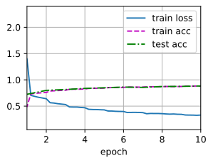
VGG网络
用块的方法实现深度神经网络
import torch
from torch import nn
from d2l import torch as d2l

def vgg_block(num_convs,in_channels,out_channels):
    layers = []
    for _ in range(num_convs):
        layers.append(nn.Conv2d(in_channels,out_channels,kernel_size=3,padding=1))
        layers.append(nn.ReLU())
        in_channels = out_channels
    layers.append(nn.MaxPool2d(kernel_size=2,stride=2))
    return nn.Sequential(*layers)
conv_arch = ((1,64),(1,128),(2,256),(2,512),(2,512))
def vgg(conv_arch):
conv_blks = []
in_channels = 1
for (num_convs,out_channels) in conv_arch:
conv_blks.append(vgg_block(num_convs,in_channels,out_channels))
in_channels = out_channels
return nn.Sequential(
*conv_blks,nn.Flatten(),
nn.Linear(out_channels * 7 * 7,4096),nn.ReLU(),nn.Dropout(0.5),
nn.Linear(4096,4096),nn.ReLU(),nn.Dropout(0.5),
nn.Linear(4096,10)
)net = vgg(conv_arch)
X = torch.randn(1,1,224,224)
for blk in net:
X = blk(X)
print(blk.__class__.__name__,'output shape:\t',X.shape)Sequential output shape: torch.Size([1, 64, 112, 112])
Sequential output shape: torch.Size([1, 128, 56, 56])
Sequential output shape: torch.Size([1, 256, 28, 28])
Sequential output shape: torch.Size([1, 512, 14, 14])
Sequential output shape: torch.Size([1, 512, 7, 7])
Flatten output shape: torch.Size([1, 25088])
Linear output shape: torch.Size([1, 4096])
ReLU output shape: torch.Size([1, 4096])
Dropout output shape: torch.Size([1, 4096])
Linear output shape: torch.Size([1, 4096])
ReLU output shape: torch.Size([1, 4096])
Dropout output shape: torch.Size([1, 4096])
Linear output shape: torch.Size([1, 10])lr,num_epochs,batch_size = 0.01,10,128
train_iter,test_iter = d2l.load_data_fashion_mnist(batch_size,resize=224)
d2l.train_ch6(net,train_iter,test_iter,num_epochs,lr,d2l.try_gpu())loss 0.287, train acc 0.894, test acc 0.887
1055.8 examples/sec on cuda:0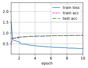
NiN模型
NiN完全取消了全连接层,使用一个NiN块,输出通道数等于标签类别数,最后放一个平均汇聚层,生成一个对数几率。
import torch
from torch import nn
from d2l import torch as d2l

def  nin_block(in_channels,out_channels,kernel_size,strides,padding):
    blk = nn.Sequential(
        nn.Conv2d(in_channels,out_channels,kernel_size,strides,padding),
        nn.ReLU(),
        # 后面两个是1x1的卷积层
        nn.Conv2d(out_channels,out_channels,kernel_size=1),
        nn.ReLU(),
        nn.Conv2d(out_channels,out_channels,kernel_size=1),
        nn.ReLU()
    )
    return blk
net = nn.Sequential(
    nin_block(1,96,kernel_size=11,strides=4,padding=0),
    nn.MaxPool2d(3,stride=2),
    nin_block(96,256,kernel_size=5,strides=1,padding=2),
    nn.MaxPool2d(3,stride=2),
    nin_block(256,384,3,1,1),
    nn.MaxPool2d(3,stride=2),
    nn.Dropout(0.5),
    nin_block(384,10,3,1,1),
    nn.AdaptiveAvgPool2d((1,1)),
    # 四维的输出转换成二维,(批量大小,10)
    nn.Flatten()
)
X = torch.rand(size=(1,1,224,224))Xtensor([[[[0.2635, 0.1056, 0.4916, ..., 0.6351, 0.0627, 0.8491],
[0.6072, 0.1263, 0.0073, ..., 0.4241, 0.0319, 0.8225],
[0.0047, 0.4005, 0.8252, ..., 0.6248, 0.6816, 0.2917],
...,
[0.2434, 0.1924, 0.9898, ..., 0.8847, 0.6104, 0.3231],
[0.4147, 0.5809, 0.0416, ..., 0.7254, 0.8195, 0.5419],
[0.2617, 0.5337, 0.8996, ..., 0.0905, 0.4162, 0.8492]]]])for layer in net:
X = layer(X)
print(layer.__class__.__name__,'output shape:\t',X.shape)Sequential output shape: torch.Size([1, 96, 54, 54])
MaxPool2d output shape: torch.Size([1, 96, 26, 26])
Sequential output shape: torch.Size([1, 256, 26, 26])
MaxPool2d output shape: torch.Size([1, 256, 12, 12])
Sequential output shape: torch.Size([1, 384, 12, 12])
MaxPool2d output shape: torch.Size([1, 384, 5, 5])
Dropout output shape: torch.Size([1, 384, 5, 5])
Sequential output shape: torch.Size([1, 10, 5, 5])
AdaptiveAvgPool2d output shape: torch.Size([1, 10, 1, 1])
Flatten output shape: torch.Size([1, 10])lr, num_epochs, batch_size = 0.1,10,128
train_iter,test_iter = d2l.load_data_fashion_mnist(batch_size,resize=224)
d2l.train_ch6(net,train_iter,test_iter,num_epochs,lr,device=d2l.try_gpu())
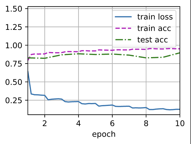
loss 0.389, train acc 0.854, test acc 0.859
4985.3 examples/sec on cuda:0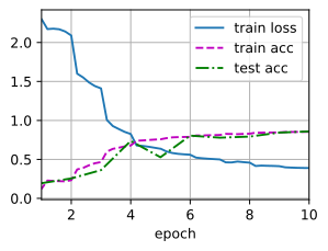
GoogLeNet
在GoogLeNet中,基本的卷积块称为$Inception$块
import torch
from torch import nn
from torch.nn import functional as F
from d2l import torch as d2l
class Inception(nn.Module):
# c1--c4是每条路径的输出通道数
def __init__(self,in_channels,c1,c2,c3,c4,**kwargs):
super(Inception,self).__init__(**kwargs)
# 路径1,单1x1卷积层
self.p1_1 = nn.Conv2d(in_channels,c1,kernel_size=1)
# 路径2,1x1卷积后接3x3卷积层
self.p2_1 = nn.Conv2d(in_channels,c2[0],kernel_size=1)
self.p2_2 = nn.Conv2d(c2[0],c2[1],kernel_size=1)
# 路径3,1x1卷积层后链接5x5卷积层
self.p3_1 = nn.Conv2d(in_channels,c3[0],kernel_size=1)
self.p3_2 = nn.Conv2d(c3[0],c3[1],kernel_size=3,padding=1)
# 路径4,3x3最大汇聚层后接入1x1卷积层
self.p4_1 = nn.MaxPool2d(kernel_size=3,stride=1,padding=1)
self.p4_2 = nn.Conv2d(in_channels,c4,kernel_size=1)
def forward(self,x):
p1 = F.relu(self.p1_1(x))
p2 = F.relu(self.p2_2(F.relu(self.p2_1(x))))
p3 = F.relu(self.p3_2(F.relu(self.p3_1(x))))
p4 = F.relu(self.p4_2(self.p4_1(x)))
return torch.cat((p1,p2,p3,p4),dim=1)
# GoogleNet实现
# 第一个模块采用64通道,7x7卷积层
b1 = nn.Sequential(
nn.Conv2d(1,64,kernel_size=7,stride=2,padding=3),
nn.ReLU(),
nn.MaxPool2d(kernel_size=3,stride=2,padding=1)
)
# 第二个模块使用两个卷积层,第一个卷积层是64通道,1x1卷积层,第二哥卷积层使用将通道数增加为3倍的3❤3卷积层
b2 = nn.Sequential(
nn.Conv2d(64,64,kernel_size=1),
nn.ReLU(),
nn.Conv2d(64,192,kernel_size=3,padding=1),
nn.ReLU(),
nn.MaxPool2d(kernel_size=3,stride=2,padding=1)
)
'''
第三个模块串联两个完整的Inception模块
* 第一个Inception块的输出通道数为64+128+32+32=256,第二条和第三条路径首先将输入通道数分别减少到96/192=1/2,和16/192=1/12,然后链接第二个卷积层
* 第二个Inception块的输出通道数增加到128+192+96+64=480,第二条路径和第三条路径先将输入通道分别减少到128/256=1/2和32/256=1/8
'''
b3 = nn.Sequential(
Inception(192,64,(96,128),(16,32),32),
Inception(256,128,(128,192),(32,96),64),
nn.MaxPool2d(kernel_size=3,stride=2,padding=1)
)
"""
第四个模块,串联5个Inception块,输出通道分别是192+208+48+64=512,160+224+64+64=512,128+256+64+64=512,112+288+64+64=528,256+320+128+128=832
"""
b4 = nn.Sequential(
Inception(480,192,(96,208),(16,48),64),
Inception(512,160,(112,224),(24,64),64),
Inception(512,128,(128,256),(24,64),64),
Inception(512,112,(144,288),(32,64),64),
Inception(528,256,(160,320),(32,128),128),
nn.MaxPool2d(kernel_size=2,stride=2,padding=1)
)
"""
第五个模块包含输出通道为256+320+128+128=832和384+384+128+128=1024的两个Inception块
后面紧跟输出层,使用全局平均汇聚层,将每个通道的高度和宽度变为1,再连接一个输出个数为标签类别数的全连接层
"""
b5 = nn.Sequential(
Inception(832,256,(160,320),(32,128),128),
Inception(832,384,(192,384),(48,128),128),
nn.AdaptiveAvgPool2d((1,1)),
nn.Flatten(),
)
net = nn.Sequential(
b1,b2,b3,b4,b5,
nn.Linear(1024,10)
)# GoogleNet模型比较复杂,可以降低输入的高度和宽度
X= torch.rand(size=(1,1,96,96))
for layer in net:
    X = layer(X)
    print(layer.__class__.__name__,'output shape:\t',X.shape)
Sequential output shape: torch.Size([1, 64, 24, 24])
Sequential output shape: torch.Size([1, 192, 12, 12])
Sequential output shape: torch.Size([1, 480, 6, 6])
Sequential output shape: torch.Size([1, 832, 4, 4])
Sequential output shape: torch.Size([1, 1024])
Linear output shape: torch.Size([1, 10])lr,num_epochs,batch_size = 0.1,10,128
train_iter,test_iter = d2l.load_data_fashion_mnist(batch_size,resize=96)
d2l.train_ch6(net,train_iter,test_iter,num_epochs,lr,d2l.try_gpu())loss 0.301, train acc 0.885, test acc 0.875
5651.3 examples/sec on cuda:0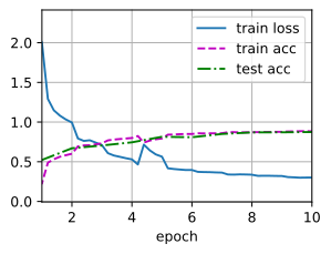
批量规范化
- 从零实现具有张量的批量规范层
import torch
from torch import nn
from d2l import torch as d2l

def  batch_normal(X,gamma,beta,moving_mean,moving_var,eps,momentum):
    # 通过is_grad_enabled方法判断当前模式是训练模式还是预测模式
    if not torch.is_grad_enabled():
        # 如果是预测模式,直接使用传入的移动平均所得的均值和方差
        X_hat = (X-moving_mean)/torch.sqrt(moving_var+eps)
    else:
        assert len(X.shape) in (2,4)
        if len(X.shape) == 2:
            # 使用全连接层的情况,计算特征维上的均值和方差
            mean = X.mean(dim=0)
            var = ((X-mean)**2).mean(dim=0)
        else:
            # 使用二维卷积层的情况,计算通道维上(axis==1)的均值和方差
            # 保留X的形状以便后面做广播运算
            mean = X.mean(dim=(0,2,3),keepdim=True)
            var = ((X-mean)**2).mean(dim=(0,2,3),keepdim=True)

        # 训练模式下,使用当前的均值和方差做标准化
        X_hat = (X - mean) / torch.sqrt(var + eps)
        # 更新移动平均的均值和方差
        moving_mean = momentum * moving_mean + (1.0 - momentum) * mean
        moving_var = momentum * moving_var + (1.0 - momentum) * var
    Y = gamma * X_hat + beta # 缩放和移位
    return Y,moving_mean.data,moving_var.data
class BatchNorm(nn.Module):
# num_features: 全连接层的输出数量或卷积层的输出通道数
# num_dims: 2表示完全连接层,4表示卷积层
def __init__(self,num_features, num_dims):
super().__init__()
if num_dims == 2:
shape = (1, num_features)
else:
shape = (1, num_features, 1, 1)
# 参与求梯度和迭代的拉伸参数和偏移参数,其分别初始化为1和0
self.gamma = nn.Parameter(torch.ones(shape))
self.beta = nn.Parameter(torch.zeros(shape))
# 非模型参数的变量初始化为0和1
self.moving_mean = torch.zeros(shape)
self.moving_var = torch.ones(shape)
def forward(self, X):
# 如果X不在内存上,将moving_mean和moving_var复制到X所在的显存上
if not self.moving_mean.device == X.device:
self.moving_mean = self.moving_mean.to(X.device)
self.moving_var = self.moving_var.to(X.device)
# 保存更新过的moving_mean和meaning_var
Y,self.moving_mean,self.moving_var = batch_normal(
X,self.gamma,self.beta,self.moving_mean,self.moving_var,eps=1e-5,momentum=0.9)
return Ynet = nn.Sequential(
nn.Conv2d(1,6,kernel_size=5),BatchNorm(6,4),nn.Sigmoid(),
nn.AvgPool2d(kernel_size=2,stride=2),
nn.Conv2d(6,16,kernel_size=5),BatchNorm(16,4),nn.Sigmoid(),
nn.AvgPool2d(kernel_size=2,stride=2),nn.Flatten(),
nn.Linear(16*4*4, 120),BatchNorm(120,2),nn.Sigmoid(),
nn.Linear(120, 84),BatchNorm(84,2),nn.Sigmoid(),
nn.Linear(84, 10)
)lr,num_epochs,batch_size = 1.0,10,256
train_iter, test_iter = d2l.load_data_fashion_mnist(batch_size)
d2l.train_ch6(net,train_iter,test_iter,num_epochs,lr,d2l.try_gpu())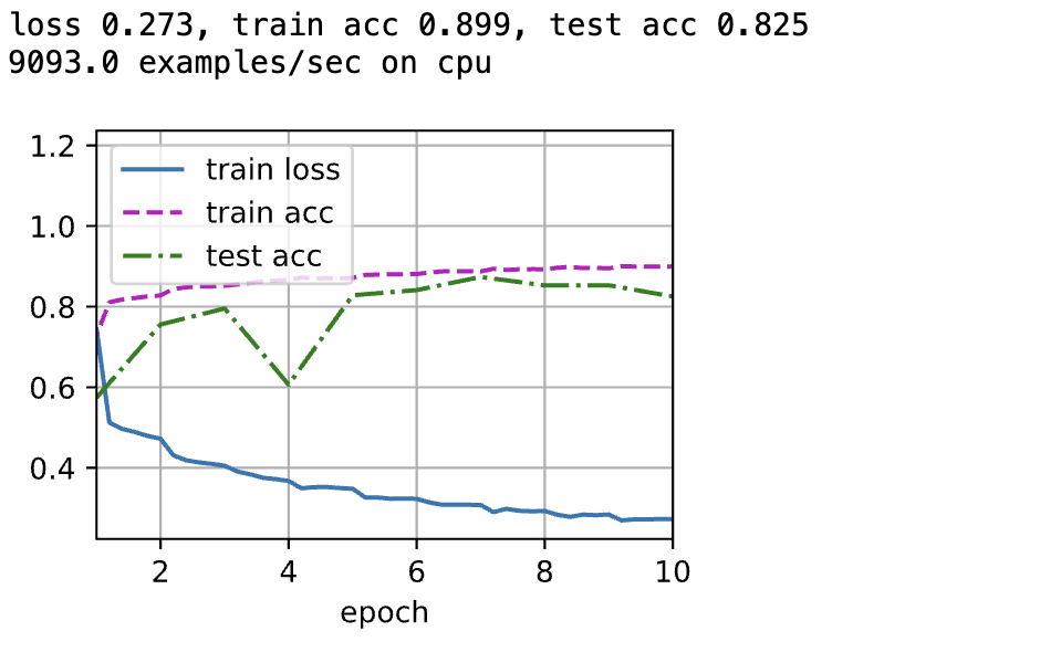
net[1].gamma.reshape((-1,)),net[1].beta.reshape((-1,))(tensor([3.0065, 3.5264, 0.6632, 2.4914, 2.3423, 3.1450],
grad_fn=<ViewBackward0>),
tensor([-3.3118, -1.7551, -0.3229, 0.2510, 1.3068, 2.4257],
grad_fn=<ViewBackward0>))简单实现
net = nn.Sequential(
    nn.Conv2d(1,6,kernel_size=5),nn.BatchNorm2d(6),nn.Sigmoid(),
    nn.AvgPool2d(kernel_size=2,stride=2),
    nn.Conv2d(6,16,kernel_size=5),nn.BatchNorm2d(16),nn.Sigmoid(),
    nn.AvgPool2d(kernel_size=2,stride=2),nn.Flatten(),
    nn.Linear(16*4*4, 120),nn.BatchNorm1d(120),nn.Sigmoid(),
    nn.Linear(120, 84),nn.BatchNorm1d(84),nn.Sigmoid(),
    nn.Linear(84, 10)
)
d2l.train_ch6(net,train_iter,test_iter,num_epochs,lr,d2l.try_gpu())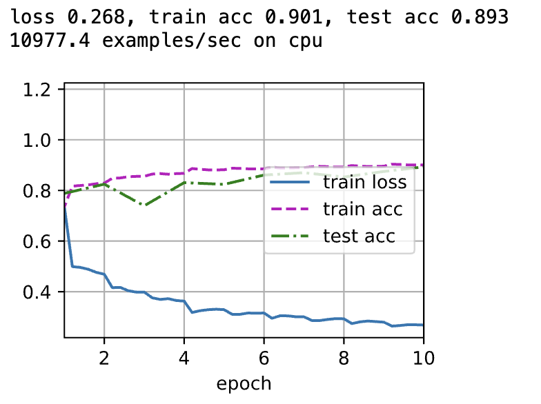
残差网络
残差块
沿用VGG的3x3卷积层设计
- 有两个相同输入输出通道数的3x3卷积层
- 每一个卷积层接一个批量规范化层和ReLU的激活函数
- 跳过两个卷积运算将输入加在最后一层ReLU的激活函数之前
- 如果要改变通道数,需要引入1x1卷积层将输入转变成所需要的形状后进行相加运算
import torch
from torch import nn
from torch.nn import functional as F
from d2l import torch as d2l

class Residual(nn.Module):
    def __init__(self, input_channels, num_channels, use_1x1conv=False, strides=1):
        super().__init__()
        self.conv1 = nn.Conv2d(input_channels, num_channels, kernel_size=3, stride=strides, padding=1)
        self.conv2 = nn.Conv2d(num_channels, num_channels, kernel_size=3, stride=1, padding=1)
        if use_1x1conv:
            self.conv3 = nn.Conv2d(input_channels, num_channels, kernel_size=1, stride=strides)
        else:
            self.conv3 = None
        self.bn1 = nn.BatchNorm2d(num_channels)
        self.bn2 = nn.BatchNorm2d(num_channels)

    def forward(self, x):
        Y = F.relu(self.bn1(self.conv1(x)))
        Y = self.bn2(self.conv2(Y))
        if self.conv3 is not None:
            x = self.conv3(x)
        # 放在最后一层激活之前
        Y = Y + x
        return F.relu(Y)
blk = Residual(3,3)
X = torch.rand(4,3,6,6)
Y = blk(X)
Y.shapetorch.Size([4, 3, 6, 6])blk = Residual(3,6,use_1x1conv=True,strides=2)
blk(X).shapeResNet模型
- 在输出通道数为64,步幅为2的7x7卷积层后,接批量规范化层,之后接步幅为2的3x3的最大汇聚层
- 使用4个由残差块组成的模块,第一个模块的通道数==输入通道数,之后每个模块的通道数是上一个模块的通道数翻倍,并将高度和宽度减半
b1 = nn.Sequential(nn.Conv2d(1,64,kernel_size=7, stride=2,padding=3),nn.BatchNorm2d(64),nn.ReLU(),nn.MaxPool2d(kernel_size=3, stride=2,padding=1))
def resnet_block(in_channels, out_channels, num_residuals,first_block=False):
    blk = []
    for i in range(num_residuals):
        if i == 0 and not first_block:
            blk.append(Residual(in_channels, out_channels, use_1x1conv=True,strides=2))
        else:
            blk.append(Residual(out_channels, out_channels))

    return blk
b2 = nn.Sequential(*resnet_block(64,64,2,first_block=True))
b3 = nn.Sequential(*resnet_block(64,128,2))
b4 = nn.Sequential(*resnet_block(128,256,2))
b5 = nn.Sequential(*resnet_block(256,512,2))net = nn.Sequential(b1,b2,b3,b4,b5,nn.AdaptiveAvgPool2d((1,1)),nn.Flatten(),nn.Linear(512,10))X = torch.rand(size=(1,1,224,224))
for layer in net:
X = layer(X)
print(layer.__class__.__name__,'output shape:\t',X.shape)Sequential output shape: torch.Size([1, 64, 56, 56])
Sequential output shape: torch.Size([1, 64, 56, 56])
Sequential output shape: torch.Size([1, 128, 28, 28])
Sequential output shape: torch.Size([1, 256, 14, 14])
Sequential output shape: torch.Size([1, 512, 7, 7])
AdaptiveAvgPool2d output shape: torch.Size([1, 512, 1, 1])
Flatten output shape: torch.Size([1, 512])
Linear output shape: torch.Size([1, 10])lr,num_epochs,batch_size = 0.05,10,256
train_iter, test_iter = d2l.load_data_fashion_mnist(batch_size)
d2l.train_ch6(net,train_iter,test_iter,num_epochs,lr,d2l.try_gpu())loss 0.126, train acc 0.951, test acc 0.897 20821.7 examples/sec on cuda:0
稠密连接网络(DenseNet)
与ResNet的关键区别在于DensNet的输出是连接,而不是相加,DenseNet这个名字由变量之间的“稠密连接”而得来,最后一层之前的所有层紧密相连。 主要组成: 稠密块(定义如何连接输入和输出) + 过渡层(控制通道数)
稠密块体
import torch
from torch import nn
from d2l import torch as d2l

def conv_block(in_channels,num_channels):
    return nn.Sequential(nn.BatchNorm2d(in_channels),nn.ReLU(),
                         nn.Conv2d(in_channels,num_channels,kernel_size=3,stride=1,padding=1))
一个稠密块由多个卷积块组成,每个卷积块使用相同数量的输出通道,在前向传播过程中,将每个卷积块的输入和输出在通道维度连接
class DenseBlock(nn.Module):
    def __init__(self,num_convs,input_channels,num_channels):
        super(DenseBlock,self).__init__()
        layers = []
        for i in range(num_convs):
            layers.append(conv_block(num_channels * i + input_channels,num_channels))
        self.net = nn.Sequential(*layers)

    def forward(self,X):
        for blk in self.net:
            Y = blk(X)
            # 连接通道维度上每个卷积块的输入和输出
            X = torch.cat((X,Y),dim=1)
        return X
blk = DenseBlock(2,3,10)
X = torch.rand(4,3,8,8)
Y = blk(X)
Y.shapetorch.Size([4, 23, 8, 8])过渡层
过渡层使用1x1的卷积层来减小通道数,并使用步幅为2的平均汇聚层减半高度和宽度
def transition_block(in_channels,num_channels):
    return nn.Sequential(nn.BatchNorm2d(in_channels),nn.ReLU(),nn.Conv2d(in_channels,num_channels,kernel_size=1),nn.AvgPool2d(kernel_size=2,stride=2))
blk = transition_block(23,10)
blk(Y).shapetorch.Size([4, 10, 4, 4])DenseNet模型
- DenseNet使用和ResNet一样的单卷积层和最大汇聚层
b1 = nn.Sequential(nn.Conv2d(1,64,kernel_size=7,stride=2,padding=3),nn.BatchNorm2d(64),nn.ReLU(),nn.MaxPool2d(kernel_size=3, stride=2,padding=1))- DenseNet使用4个稠密块,设置每个稠密块使用4个卷积层,卷积层通道数为32,所以每个稠密块将增加128个通道数
- 模块之间,DenseNet使用过渡层减半高度和宽度
num_channels,growth_rate = 64,32
num_convs_in_dense_blocks = [4,4,4,4]
blks = []
for i,num_convs in enumerate(num_convs_in_dense_blocks):
    blks.append(DenseBlock(num_convs,num_channels,growth_rate))
    # 上一个稠密块的输出通道
    num_channels += num_convs * growth_rate
    # 在稠密块之间添加一个过渡层,使通道数减半
    if i!=len(num_convs_in_dense_blocks)-1:
        blks.append(transition_block(num_channels,num_channels // 2))
num_channels //= 2- 与ResNet类似,最后连接全局汇聚层和全连接层来输出结果
net = nn.Sequential(b1,*blks,nn.BatchNorm2d(num_channels),
                    nn.ReLU(),
                    nn.AdaptiveAvgPool2d((1,1)),
                    nn.Flatten(),
                    nn.Linear(num_channels,10))
lr,num_epochs,batch_size = 0.1,10,256
train_iter, test_iter = d2l.load_data_fashion_mnist(batch_size,resize=96)
d2l.train_ch6(net,train_iter,test_iter,num_epochs,lr,d2l.try_gpu())loss 0.140, train acc 0.949, test acc 0.904
9091.2 examples/sec on cuda:0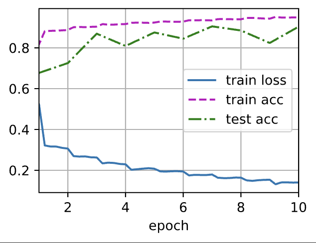
留言讨论
0 条留言
正在加载留言...